“Electric Vehicle Population Data” from the U.S. Department of Energy, available on Data.gov. (https://catalog.data.gov/dataset/electric-vehicle-population-data)
“Washington State Population and GDP Per Capita Data” from Bureau of Economic Analysis, U.S. Department of Commerce, available on bea.gov. (https://www.bea.gov/)
“Personal Consumption Data in Washington State” from from Bureau of Economic Analysis, U.S. Department of Commerce, available on bea.gov. (https://apps.bea.gov/regional/downloadzip.cfm)
(2) Data Descriptions:
These datasets are collected and maintained by the U.S. Department of Energy and Department of Commerce, reflecting the statistics on electric vehicle ownership in Washington state, as well as the economic factors.
The data is available in CSV format, which is convenient for importing and analyzing in most data analysis tools.
The dataset is updated regularly, ensuring access to the latest trends and numbers.
It includes key information such as the make and model of the vehicle, the type of electric vehicle, geographical data, and basic socio-economic data of Washington State.
(3) Potential Issues with Data:
Initial review suggests the data is comprehensive but will require a thorough quality check for inconsistencies or inaccuracies.
(4) Import Method:
The data will be imported using the read.csv function from R’s built-in utilities. Additional R packages like dplyr and tidyr may be utilized for data manipulation and cleaning, ensuring that the dataset is in the optimal format for analysis.
2.2 Research Plan
(1) Analyzing Trends in EV Adoption:
Time-Series Analysis: We will conduct a time-series analysis to understand how the popularity of electric vehicles has evolved over the years. By plotting the number of EVs registered each year, we can identify trends, growth rates, and potential inflection points in EV adoption.
Comparative Analysis: By comparing the adoption rates of different types of EVs (eg. hybrids vs. fully electric), we can gain insights into consumer preferences and technological advancements in the field.
(2) Investigating Geographical Variations:
Spatial Analysis: Using the geographical data available in the dataset, we will conduct a spatial analysis to map out the distribution of EVs across WA.
Correlation with External Factors: We’ll explore correlations between EV adoption and external factors such as state-level policies on EVs, charging infrastructure availability, and socio-economic indicators. This will help us understand the driving forces behind regional differences in EV adoption.
(3) Exploring Vehicle Types:
Categorization and Frequency Analysis: The dataset will be categorized based on vehicle types. We will perform a frequency analysis to determine the most popular types of EVs.
Cross-Tabulation with Other Variables: By cross-tabulating vehicle types with other variables like geographical location and year of registration, we can uncover deeper insights into the market dynamics and consumer preferences.
2.3 Missing value analysis
Code
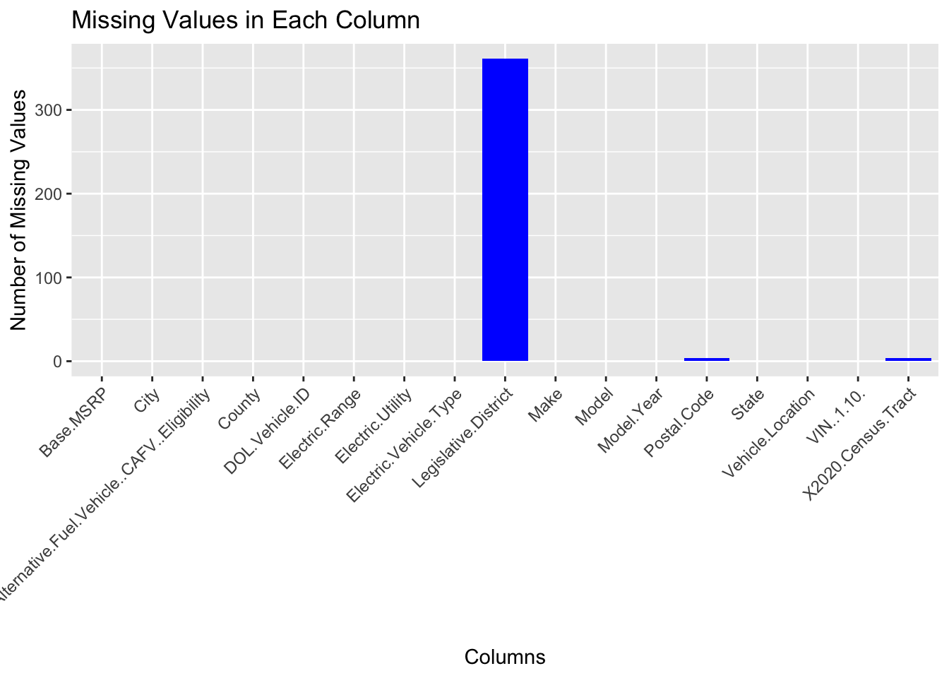
library(ggplot2)suppressPackageStartupMessages(library(reshape2))suppressPackageStartupMessages(library(dplyr))ev_data <-read.csv('/Users/hujiasheng/Electric_Vehicle_Population_Data.csv')missing_values <-sapply(ev_data, function(x) sum(is.na(x)))# Filter out columns with no missing values for plotting#missing_values <- missing_values[missing_values > 0]missing_df <-data.frame(Column =names(missing_values), MissingCount = missing_values)ggplot(missing_df, aes(x = Column, y = MissingCount)) +geom_bar(stat ="identity", fill ="blue") +theme(axis.text.x =element_text(angle =45, hjust =1)) +ggtitle("Missing Values in Each Column") +xlab("Columns") +ylab("Number of Missing Values")
Code
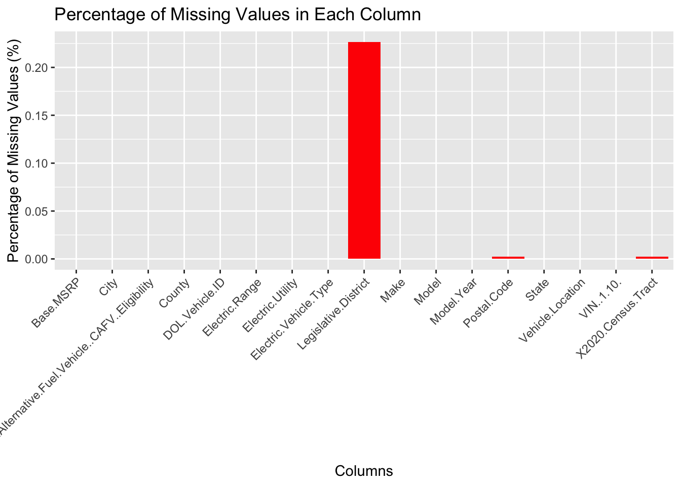
total_rows <-nrow(ev_data)missing_percentage <- (missing_values / total_rows) *100missing_percent_df <-data.frame(Column =names(missing_percentage), MissingPercent = missing_percentage)ggplot(missing_percent_df, aes(x = Column, y = MissingPercent)) +geom_bar(stat ="identity", fill ="red") +theme(axis.text.x =element_text(angle =45, hjust =1)) +ggtitle("Percentage of Missing Values in Each Column") +xlab("Columns") +ylab("Percentage of Missing Values (%)")
The analysis of the Electric Vehicle Population Data reveals insightful patterns regarding missing values, as depicted in the following two graphs
Missing Values Count: The first graph displays the count of missing values in each column where missing values are present. This graph provides a clear indication of which columns have missing data and the extent of these missing values.
Percentage of Missing Values: The second graph shows the percentage of missing values relative to the total number of rows in the dataset for each column with missing data. This perspective is crucial for understanding the significance of the missing data in relation to the entire dataset.